Barbara, our neighbor who has lived here for several decades, very kindly invited me to photograph two of her historic maps of this locality, one from 1876 and the other from 1881. The maps show roads, buildings and significant topographic features such as hills, aqueducts and railways.
I wanted to overlay the photographs of the old maps with current assessor’s parcel maps in order to easily see how the neighborhood has changed over time. The process of turning a photograph into a properly oriented map layer in a geographic information system is called “registration, rectification and warping” the image. The process involves comparison of points on the photographed map that are still identifiable on current maps. The process is to match individual pixels in the photograph to the coordinates of the real-world location that they correspond to on the current map. Whit these “ground control points” established, various software can then rotate, resize and “warp” the photographed map into approximate alignment with the current map. This enables both old and new to appear together or in a time sequence, without requiring any adjustment of the maps from one time period to another.
I decided to register, rectify and warp my two historic map images using a software package called the Geographic Resources Analysis Support System (or, GRASS), a free and open-source product with an active user and developer community. Unfortunately, although GRASS has many potentially useful and powerful capabilities, it was originally designed as a command-line tool (meaning users typed text commands, one at a time, to accomplish their work) rather than with more user-friendly graphical user interface. And, as still seems endemic in the free and open-source world, most documentation is oriented toward developers or users already familiar with the software’s core concepts. So, if I am able to figure out how to use GRASS to perform registration, rectification and warping, I’ll want to have some good directions available next time around; this blog post will serve that purpose. (Non-technical readers need go no further.)
The “raw” (unregistered, unrectified, unwarped) data in this example is the photo of Barbara’s historic map, which starts as a collection of pixels in rows and columns, each with a color value. Seen together, they look like a map image. None of the pixels contain any coordinate information about the real-world location they represent. I need data about the same area covered by the historic map, but with real-world coordinates available. A public site with free assessor’s parcels for our town had exactly this in an ESRI shapefile format. I downloaded the parcel data for our town and stored it in a directory along with the images of Barbara’s maps (in PNG format).
Next, I opened GRASS, and was presented with a “Weldome to GRASS GIS” screen that included a button called “Location Wizard” for defining a new location. In GRASS, locations are user-defined regions and resolutions that influence how some of the GRASS commands work. To do much of anything in GRASS, you have to deine a location. So, I stepped through the screens provided by the wizard, including setting North, South, East and West coordinates for the region of interest and specifying a map projection. I left the grid resolution at the default of 1.0 and 1.0 and called the new Location “my_neighborhood”.
Next, at the same Welcome screen, I clicked the “Create mapset” button and named the new mapset “my_mapset”. For a task that only I will be performing (hopefully) once on a single dataset, mapsets aren’t very relevant, as their purpose is to manage multiple user edits of the same datasets. However, to avoid confusion or some unexpected GRASS requirements, I’m going through the motions.
Then I clicked the button saying “Start GRASS” and three windows opened: a terminal with a GRASS command line, a Layer Manager and a Map Display. In the Layer Manager window’s menu, I selected File -> Import Vector Map -> Multiple Import Formats using OGR. The resulting dialog window had multiple tabs, so I went through all of them and identified the parcel shapefile dataset in the “OGR datasource name” field and called it “parcels” in the “Name for output vector map” field. The shapefile’s projection already matched that of the Location I had just created.
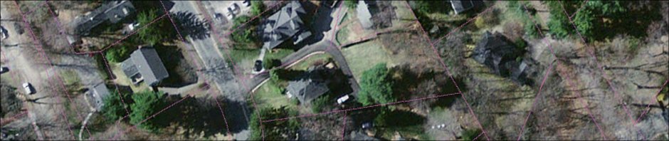
The parcels loaded as intended, which I was able to prove by clicking on the second icon from the left in the Layer Manager named “Load map layers into workspace” and then clicking the refresh icon in the Map Display window. The restul looked like this:
 Thus far, the steps have established a data environment in GRASS that will provide real-world coordinate information about my neighborhood. Next comes the “raw” map photo from Barbara.